| dc.description.abstract | Topic: Frequency counts, risk analysis
Context:
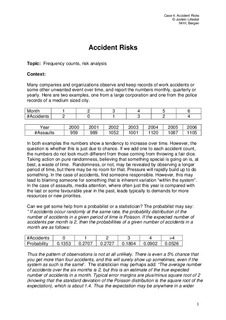
Many companies and organizations observe and keep records of work accidents or some other unwanted event over time, and report the numbers monthly, quarterly or yearly. Here are two examples, one from a large corporation and one from the police records of a medium sized city.
Month 1 2 3 4 5 6
#Accidents 2 0 1 3 2 4
Year 2000 2001 2002 2003 2004 2005 2006
#Assaults 959 989 1052 1001 1120 1087 1105
In both examples the numbers show a tendency to increase over time. However, the question is whether this is just due to chance. If we add one to each accident count, the numbers do not look much different from those coming from throwing a fair dice. Taking action on pure randomness, believing that something special is going on is, at best, a waste of time. Randomness, or not, may be revealed by observing a longer period of time, but there may be no room for that. Pressure will rapidly build up to do something. In the case of accidents, find someone responsible. However, this may lead to blaming someone for something that is inherent variation “within the system”. In the case of assaults, media attention, where often just this year is compared with the last or some favourable year in the past, leads typically to demands for more resources or new priorities.
Can we get some help from a probabilist or a statistician? The probabilist may say:
” If accidents occur randomly at the same rate, the probability distribution of the number of accidents in a given period of time is Poisson. If the expected number of accidents per month is 2, then the probabilities of a given number of accidents in a month are as follows:
#Accidents 0 1 2 3 4 >4
Probability 0.1353 0.2707 0.2727 0.1804 0.0902 0.0526
Thus the pattern of observations is not at all unlikely. There is even a 5% chance that you get more than four accidents, and this will surely show up sometimes, even if the system as such is the same”. The statistician may perhaps add: “The average number of accidents over the six months is 2, but this is an estimate of the true expected number of accidents in a month. Typical error margins are plus/minus square root of 2 (knowing that the standard deviation of the Poisson distribution is the square root of the expectation), which is about 1.4. Thus the expectation may be anywhere in a wider region around 2, so that any claim that the 4 accidents last month are due to increased hazards is even more unjustified”.
You have taken a course in statistics in school, and have been taught about hypothesis testing, and you wonder whether this can be used. There are some problems: (i) It assumes a “true” expected rate and independent random variation, (ii) it typically compares expectations in one group of data with a hypothesized value, or with other groups of data. Here we have just instants, (iii) it may neglect the order of the data and may not pick up trends, and (iv) it does not handle the monitoring over time in an attractive manner. These objections may be remedied by more sophisticated modelling, but becomes unattractive for common use.
You may also have heard about statistical process control, and the use of control charts to point out deviant observations. This keeps track of the order of observations and may also react to certain patterns in the data, like level shifts and increasing trends. The drawback is: (i) it assumes at the outset a stable system (a process in “statistical control”) and the monitoring of deviant observations and patterns (ii) the data requirements are in many cases demanding. In practice we often do not have a stable system, things change over time, from year to year, and we do not have enough data to establish the control limits, even if the system was stable.
Avoiding the reaction to deviant observations which are just random is a big issue in quality management, since it typically leads to more variation and turbulence in the system. This is justified in a context where you ideally have a system, stable over time, and running according to fixed procedures (until they are changed), e.g. in a production context and for some administrative processes. You may also have this in some contexts closely related to human hazards, say monitoring birth defects.
We probably have to realize that in many situations related to hazards there is no stable system and cannot be, and that some kind of reaction is required before we know the truth. What then to do? If we ask a risk analyst, he or she may be stuck in the traditional statistical theory, while others have dismissed traditional statistical theory as basis for active risk management (see Aven: Risk Analysis, 2003). Data of the kind above occur frequently, and there is room for a more pragmatic attitude. Otherwise the data will either be neglected, because no one can tell how to deal with them in a systematic manner (and particularly so the statisticians) or they will be misused for opportunistic purposes.
One possibility for monitoring with the aim to pick up trends in short series is described in Kvaløy & Aven (2004). It is slightly modified here (see next page) and is easily programmed in Excel:
Theory
A sequence of hazards for r consecutive periods is given, and the objective is to point out a worsening trend or individual hazards that are aberrant. Do the following:
1. Calculate the average mj of the observed hazards up to and including period j
2. Take ej = (r-j)mj as expected number of hazards for the remaining r-j periods
3. Use the Poisson distribution with expectation ej to calculate the probability that the number of hazards for the r-j remaining periods is at least as observed
4. If this probability is small, say less than 5% then initiate warning or alarm.
Repeat 1-4 for all or some of j = r-1 , r-2 ,…,1
Note: If the counts are very high, we may use the normal distribution with expectation ej
and standard deviation the square root of ej instead.
The first example above gives this calculation scheme for judgment at month six:
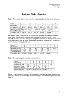
Month 1 2 3 4 5 6
#Accidents 2 0 1 3 2 4
Average till now 2.0 1.0 1.0 1.5 1.6 2.0
Expected ahead 10.0 4.0 3.0 3.0 1.6 -
Observed ahead 10 10 9 6 4 -
Probability (tail) 0.5421 0.0081 0.0038 0.0840 0.0788 -
We see that alarm is given at this month, due to some small tail probabilities looking ahead from month two and three. The 4 in the sixth month (observed ahead from the fifth) is not that surprising, judged from the average of the preceding. Neither is the combined 6 of two last months judged from the average of the preceding. However, the combined 9 of the last three months is dubious compared with the average of the preceding, and so is the case moving one additional month backward. Going all the way back to month 1 we have just one single observation 2 and then “expect” 10 altogether for the 5 months ahead, and that is exactly what we got, thus leading to a high tail probability.
Task 1: Replace the number 4 of the sixth month with 3 and repeat the analysis.
Task 2: Analyse the data available after five months, i.e. omit month 6.
Task 3: Use the described method to analyse the second example | nb_NO |