| dc.description.abstract | Topics:
One-sample and two-sample estimation and testing, analysis of variance and regression
Context:
The users of a data base system, e.g. in a bank, will emphasize short response times when searching the data base. The response time may vary, depending on the type of search, the number of simultaneous searching and technical circumstances related to the transmission of data. Response times over a threshold lead to irritation and delay. This threshold is typically between 5 and 10 seconds, but varies between individuals. The response times are occasionally much longer, caused by traffic getting stuck.
It is possible to generate fictitious requests which can be followed through the system in order to uncover “bottlenecks”. It is also possible to make minor modifications on the system, both with respect to programming and technical solutions, so that efficiency comparisons can be made.
A fictitious request every 5th minute, i.e. 72 within the common working hours from 9.30 a.m. to 3.30 p.m. is few in comparison with the total number of requests of about 5000, and will therefore have a negligible effect on the response times of the system. We have data from Wednesdays in two consecutive weeks (Day 1 and Day 2), with a system they change in between, intented to reduce response times. The effect can be judged by various criteria: the change in expected response time, the change in median response time or by a change of the chance that the response time exceeds a certain “critical” level ,say 5 seconds.
Data are available in the file Respose_Times.XLS as follows:
Response time (in seconds)
Day (1-2)
Hour (1-6)
Lunch break (0-1)
Traffic (no. of requests in encompassing minute)
How the data will be analyzed depends on how much statistical theory you have. In particular some distribution theory beyond the normal distribution may be helpful.
Task (A-version):
What can be said about response times before and after the system change?
Can we conclude that the system change led to an improvement?
Task (B-version)
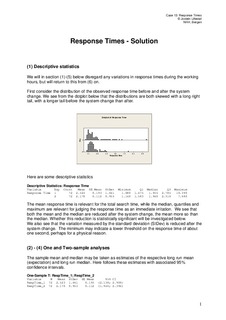
1. Present the distribution for the sampled response times for each Wednesday separately, and comment on their shape and possible differences.
2. Estimate, before and after the system change
a. the mean response time.
b. the median response time.
c. the probability that the response time exceeds 5 seconds
If you can, provide sampling error limits to each estimate..
3. Estimate the difference of (before minus after)
a. the mean response times.
b. the median response times.
c. the probabilities that the response time exceeds 5 seconds
If you can, provide sampling error limits to each estimate.
4. Perform the standard formal tests of the hypothesis of no change in 3 a, b and c.
Which one of the tests is most relevant for our problem?
Are the assumptions for these tests satisfied?
5. *Make a reasonable assumption for the distribution of the random response time T.
Do the following after the system change:
a. Estimate the parameters of the model and compute an estimate of .
b. Estimate the maximal response time that can be guaranteed with 95% certainty.
Hint: A possibility is to set T = a + X, where a is the smallest possible response time,
and let the overshoot X be distributed Gamma or lognormal.
What can be said in favour and disfavour of assuming a specific distribution?
6. It may be that the response times vary over the day, and that this may affect the analysis above. A possibility is to pair the observations for the same time the two Wednesdays, and then analyse the 72 differences in response time (before minus after). Estimate
a. the expected difference in response times,
b. the median difference in response times,
c. the probability of a shortened response time after the system change
7. Perform the standard formal tests of the hypothesis of no change in 6.
Hint: One-sample T-test, one-sample rank test, sign-test. Discuss the choice of test for this data.
Comment on the result of the testing, and whether the pairing of observations may reduce the possibility of testing improvement with respect to unacceptable response times.
Do you see an alternative if the number of requests in the lunch break from 11.30 to 12.30 are typically shorter.
8. Figure out whether the response times vary over the day by
a. making suitable plots
b. one-factor analysis of variance (ANOVA) for the Day 1 observations using Hour (1-6) as factor.
c. two-factor analysis of variance (ANOVA) all observations using Hour (1-6) as the first factor and Day (1-2) as the second factor.
9. As a measure of the traffic it is recorded the number of requests in the minute encompassing each fictitious request. Analyse by regression analysis how the traffic affects the response times, and whether there is improvement from Day 1 to Day 2. Discuss whether the standard assumptions for regression analysis are fulfilled.
An underlying assumption for some of the analysis above is independent observations. Discuss the possibility of positive correlation, and the risk that this may twist our conclusions.
10. *Study the relationship between traffic and response times over 5 seconds by logistic regression
11. *It is claimed that the number of requests in a given period is Poisson distributed. Is this reasonable or unreasonable? Can this assumption be tested?
For planning purposes the expected number of requests pr. minute is set to 16. Is this reasonable? Compute approximate the probability that the number of requests pr. minute is more than 25. | nb_NO |